
7 Digital Controller Design
7.10 Design ExampleAll Activities
The following design example illustrates the state-space design concepts discussed in the textbook.
You can change some of the design parameters in this example. The example will then update the calculations and results. Update the design values using the controls in the example or the duplicates here
Consider the inverted pendulum on a cart driven by a position servo as shown in Figure 1.
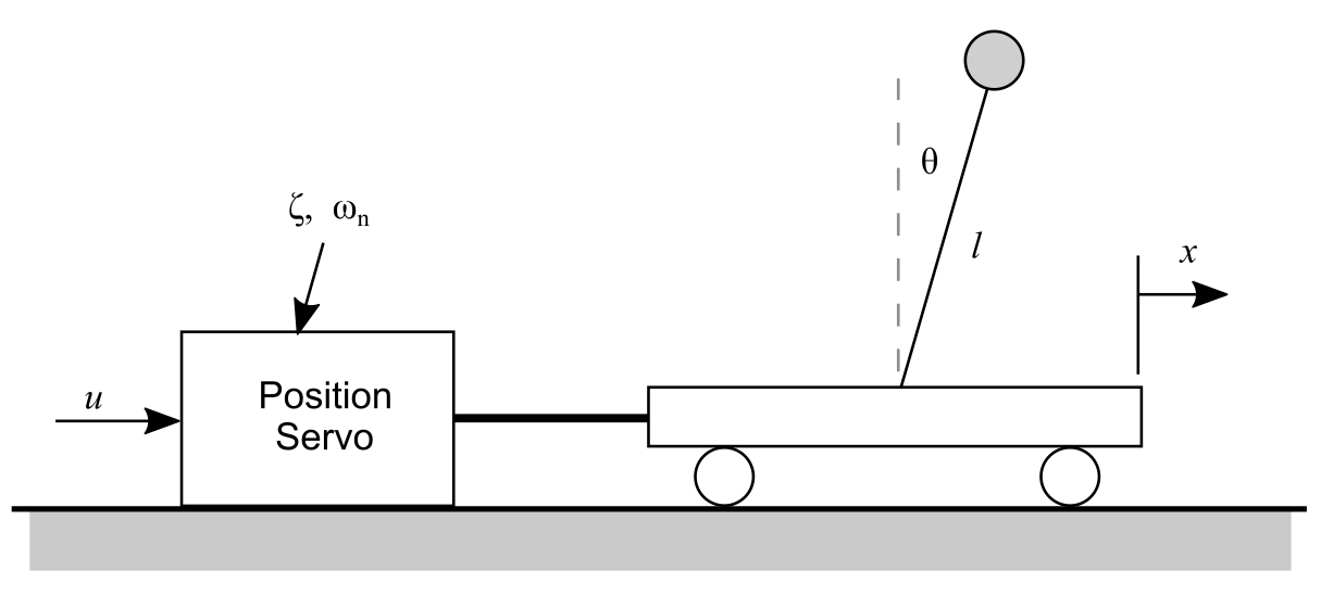
The equation of motion of the pendulum is
$$\ddot{x}+l\ddot{\theta}-g\theta = 0$$and the cart is
$$\ddot{x} + 2\zeta\omega_n\dot{x} + \omega_n^2x = \omega_n^2u$$where $u$ is the input to the position servo.
Eliminate $\ddot{x}$ using both equations of motion, and one gets
$$\ddot{\theta}=\frac{g}{l}\theta+ \frac{\omega_n^2}{l}x+\frac{2\zeta\omega_n^2}{l}\dot{x}-\frac{\omega_n^2}{l}u$$Pick the state vector
$$\bold{x}= \begin{bmatrix} x_1\\x_2\\x_3\\x_4 \end{bmatrix} = \begin{bmatrix} \theta\\ \dot{\theta} \\ x \\ \dot{x} \end{bmatrix}$$then the following system and input matrices obtain:
$$ \bold{A} = \begin{bmatrix} 0 & 1 & 0 & 0 \\ g/l & 0& \omega_n^2/l & 2\zeta\omega_n/l \\ 0 & 0 & 0 & 1 \\ 0 & 0 & -\omega_n^2 & -\zeta\omega_n \end{bmatrix}, \optbreak{} \bold{B}= \begin{bmatrix} 0\\ -\omega_n^2/l \\ 0 \\ \omega_n^2 \end{bmatrix} $$
Numerical Values.
To go any farther we need some numerical values. For the pendulum $$\begin{aligned} g &= 9.8 \text{m/sec}^2 \\ l &= 0.3 \text{m} \end{aligned}$$To go any farther we need some numerical values. For the pendulum
$$\begin{aligned} \zeta &= 0.707 \\ \omega_n &= 20 \text{rad/sec} \end{aligned}$$and we get plant matrices
$$\bold{A}= \begin{bmatrix} 0 & 1 & 0 & 0\\ 32.7 & 0 & 1333 & 94.3 \\ 0 & 0 & 0 & 1\\ 0 & 0 & -400 & -28.3 \end{bmatrix}, \optbreak{} \bold{B} = \begin{bmatrix} 0 \\ -1333 \\ 0 \\ 400 \end{bmatrix}$$Since the position servo natural frequency is about 3 Hz, we won’t require any higher frequency response from the controlled system. Thus a sampling frequency of 25 Hz ($T$ = 0.04) should be adequate. Discretizing the plant with this $T$ yields
$$ \bold{\Phi} = \begin{bmatrix} 1.0262 &0.0403 & 0.7240 & 0.0619\\ 1.3181 & 1.0262 & 29.0507 & 2.7782 \\ 0 & 0 & 0.7839 & 0.0215\\ 0 & 0 & −8.6106 & 0.1751 \end{bmatrix} , \optbreak{} \bold{\Gamma} = \begin{bmatrix} −0.7240 \\ −29.0507 \\ 0.2161 \\ 8.6106 \end{bmatrix}$$
Step Response of Plant.
As a "reality check," find the response of the pendulum to a step position input of 1 cm (0.01 m). Selecting $\bold{C} = \begin{bmatrix} 1&0&0&0 \end{bmatrix} $ to yield $\theta$ as the output, we obtain the pendulum angular response shown in Figure 2. The pendulum angle of Figure 2 looks believable, it is in the negative direction which is consistent with our intuition for a positive base displacement.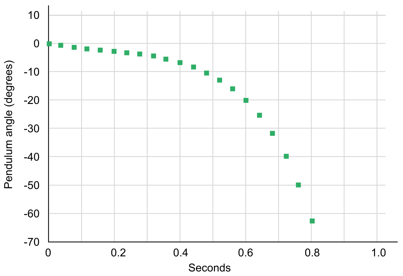
Plant Controllability.
Before continuing on with the controller development, check that the plant is controllable with the given input. By adjusting the base position, it seems obvious that it is possible to control both base position and velocity, and pendulum position and velocity. Nevertheless, intuition can be in error, and it is best to check.
  Phi = [1.0262 1.3181 0 0;

  0.0403 1.0262 0 0;

  0.7240 29.0507  0.7839  −8.6106;

  0.0619  2.7782 0.0215  0.1751];

  Gamma = [−0.7240; −29.0507; 0.2161; 8.6106];
    Ctr = ctrb(Phi,Gamma);

rank(Ctr)
MATLAB will display:
ans = 4
As expected, the plant is controllable.
Control Law.
In keeping with , Butterworth filter guidelines Given filter order $n$, poles are at $$s_k = \omega_n e^{\frac{j(2k_n-1)}{2n}} \text{ for }k=1,2,3, \dots,n $$ equally space four poles at radius $\omega_k$ around the negative real axis in the s-plane hence at angles of $\pm 22.5\degree, \pm67.5\degree$ from the negative real axis.For $\omega_K$ = rad/s (A logical choice is $\omega = \omega_n$ = 20rad/s)
The four poles in the s-plane are: .
In the z plane these four poles are: .
Using Matlab place, the state feedback gain is
Plant Observability.
Assume that only a measurement of pendulum angle is available (measurement of cart position is probably available, since its position is controlled), can we estimate the full state vector from only a measurement of pendulum angle? The $\bold{C}$ matrix will be $$\bold{C} = \begin{bmatrix} 1 & 0 & 0 & 0 \end{bmatrix}$$and a check of the observability matrix shows
  C = [1 0 0 0];

    rank(ctrb(Phi',C'));
MATLAB will display:
ans = 4
Since the observability matrix has full rank, the system is observable, and we can proceed with a prediction estimator design.
Prediction Estimator
Place the estimator poles like the previous control law poles, but use a higher natural frequency of $\omega_L$For $\omega_L$ = rad/s
The four poles in the s plane are: .
In the z plane these four poles are: .
Reference Input.
We wish to specify the position of the cart using the reference input, or $y_r = x$. This is a different variable than the measurement $\theta$, so $\bold{C}_r \ne \bold{C}$, and $$\bold{C}_r = \begin{bmatrix} 0 & 0 & 1 & 0 \end{bmatrix}$$It doesn’t really make sense to provide a reference input for pendulum angle $\theta$, except for trimming, since $\theta = 0$ is the only pendulum angle that can exist in steady-state. So the number of plant inputs $u$ and desired outputs $x$ are the same ($m = p$), hence the coefficient matrix in equation (7.70) is square, and terms $\bold{N}_x$ and $N_u$ are given by equation equation (7.71) $$\tag{7.71} \begin{bmatrix}\bold{N}_x \\ \bold{N}_u \end{bmatrix} = \begin{bmatrix}\bold{\Phi}-\bold{I} & \bold{\Gamma} \\ \bold{C}_r & \bold{0} \end{bmatrix}^{-1} \begin{bmatrix} \bold{0} \\ \bold{I} \end{bmatrix}$$ (See Section 7.8.1 in the textbook))
    Cr = [0 0 1 0];

    inv([Phi-eye(4) Gamma ; Cr 0])*([0;0;0;0;1])
MATLAB will display:
      ans = -0.0000

             0.0000

             1.0000

             0.0000

             1.0000
Thus
$$\bold{N}_x = \begin{bmatrix} 0\\0\\1\\0 \end{bmatrix}, N_u=1$$
System Modeling.
The complete system is modeled by the five following equations (integrated in the proper manner, of course!): $$\begin{aligned}\bold{x}(k+1) &= \bold{\Phi x}(k) + \bold{\Gamma}u(k)\\ y(k) &= \bold{Cx}(k)\\ \bold{\hat{x}}(k+1) &= \bold{\Phi \hat{x}}(k) + \bold{\Gamma}u(k) + \bold{L}[y(k) - \bold{C \hat{x}}(k)] \\ u(k) &= -\bold{K}[\bold{\hat{x}}(k) - \bold{x}_r(k)] + N_ur(k) \\ \bold{x}_r(k) &= \bold{N}_xr(k) \end{aligned}$$
Initial Condition Response.
First impose an initial condition on the plant and observe its return to equilibrium. Note that this controller will return all four states to equilibrium... it will balance the stick and also center the cart. Let’s pick an initial offset of 0.01 m (1 cm) for the cart, with the pendulum balanced, hence $$\bold{x}(0) = \begin{bmatrix} \theta_0 \\ \dot{\theta}_0 \\ x_0 \\ \dot{x}_0 \end{bmatrix} = \begin{bmatrix} 0\\ 0\\ 0.01 \\ 0 \end{bmatrix}$$The response of the cart position and pendulum angle as the system returns to equilibrium is shown in Figure 3. Note that the initial motion of the cart is to the right, away from the desired center position! However, this is intuitive, since the stick was initially balanced, and to move the cart back to the left one must first move to the right to get the stick leaning to the left, then the cart can move left.
Reference Input Response.
Our reference input acted on cart position, thus we can specify reference cart position and the other variables will be regulated. Choose cart motion of 0.2 m (20 cm) in 1 second (25 samples) at constant velocity. The system behavior to this reference trajectory appears in Figure 4, where again cart position and pendulum angle are plotted. As before, the cart moves the "wrong way" first, then moves back in the desired direction.The previous example uses an estimator to predict the states and then uses those estimates, $\bold{\hat{x}}$, to calculate the feedback control, $u=\bold{K\hat{x}}$. In the example, it was assumed that we knew the plant exactly. This means the estimator can predict the state values perfectly. It also means that the feedback control gain, $\bold{K}$, will place the closed-loop poles exactly as designed. However, we are rarely able to model systems perfectly. A good control system must be "robust" and work even if the actual plant varies slightly from the model used in the design.
Use control below to change the value of the pendulum length. The example above will use the nominal length, 0.3m, for the design calculations, but the simulation will use the longer pendulum length.
Update the design values using the controls in the example or the duplicates here
- Use the nominal pendulum length. Vary the value for $\omega_L$. This changes the "speed" of the estimator. Observe the response in Figure 3. How does this change affect the system performance and why?
- Change the actual pendulum length to ½% longer. Vary the value for $\omega_L$. This changes the "speed" of the estimator. Observe the response in Figure 3. How does this change affect the system performance and why?
- Change the actual pendulum length to 1% longer. Vary the value for $\omega_K$. This changes the "speed" of the closed-loop poles. Observe the response in Figure 3. How does this change affect the system performance and why?