7 Design with SS

NOTE: This example allows you to change design values. Results will be automatically updated on-the-fly. Results in the example are calculated at a lower precision than used by MATLAB so values displayed on this example may vary slight from those calculated directly using MATLAB. When in doubt, use MATLAB's values.

Values can be changed using the controls in the example or duplicates here

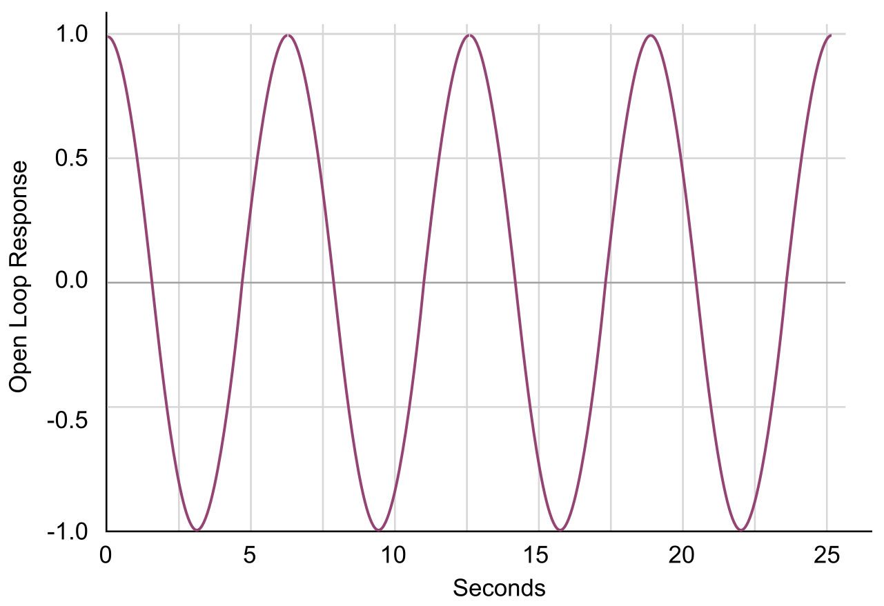
In this example a control law and estimator will be designed for an undamped 1 rad/sec harmonic oscillator. The plant transfer function is

$$\frac{Y(s)}{U(s)} = \frac{1}{s^2+1}$$

with differential equation $\ddot{y} + y = u$. Using state vector

$$\bold{x}=\begin{bmatrix}x_1 \\ x_2 \end{bmatrix} = \begin{bmatrix} y \\ \dot{y} \end{bmatrix}$$

we have plant matrices

$$\bold{A}=\begin{bmatrix}0 & 1\\ -1 & 0 \end{bmatrix}, \bold{B}=\begin{bmatrix}0 \\ 1 \end{bmatrix} ,\optbreak{} \bold{C} = \begin{bmatrix} 1 & 0 \end{bmatrix}, D=0$$

The response of this plant from initial condition (1,0) is shown in Figure 1.

Specifications

One option is to increase the damping to critical while keeping the same natural frequency of 1 rad/sec. Those desired pole locations would be at $s = -1, -1$. Set

Sampling period

At the chosen poles, the controlled system will have natural frequency of approximately 1 rad/sec, or about 1 Hz. Acceptable practice is to pick a sampling frequency to be approximately five to ten times this frequency. Choose T = second.

Plant Discretization

Using this $T$, the continuous plant can be defined, then discretized using MATLAB:

A = [0 1;-1 0];
B = [0;1];
C = [1 0];
D = 0;
plant_c = ss(A,B,C,D);
T = 1;
plant_d = c2d(plant_c,T)

MATLAB will display:

a =
           x1       x2
  x1   0.5403   0.8415
  x2  -0.8415   0.5403

b =
           u1
  x1   0.4597
  x2   0.8415

c =
      x1    x2
  y1   1     0

d =
      u1
  y1   0

Sampling time: 1
Discrete-time model.

Note that the state-space matrices can be extracted from LTI model plant d by:

Phi = plant_d.A
Gamma = plant_d.B

MATLAB will display:

Phi =
   0.5403   0.8415
  -0.8415   0.5403

Gamma =
   0.4597
   0.8415

Control Law

The desired z-plane pole locations are found using the mapping $z = e^{sT}$,

control_s_poles = [-1 -1]';
control_z_poles = exp(control_s_poles*T)

MATLAB will display:

control_z_poles =  0.3679
                   0.3679

It is a numerical anomaly of MATLAB function place that poles of multiplicity greater than the number of inputs are not allowed. One pole can therefore be offset slightly, and the gain vector $\bold{K}$ is

control_z_poles(1) = control_z_poles(1)+0.0001;
K = place(Phi,Gamma,control_z_poles)

MATLAB will display:

place: ndigits= 19
K = -0.5655  0.7186

The control law $u = −\bold{Kx}$ is seen to be positive position feedback and negative velocity feedback. As a check, simulate the controlled system response from initial condition (1,0). This is shown in Figure  2.

Initial condition response

Prediction Estimator

For the original design select the natural frequency of the prediction estimator to be five times the controlled plant, again with critical damping. For that case the estimator pole locations would be $s = −5,−5$. Set

estimator_s_poles = [-5 -5]';
estimator_z_poles = exp(estimator_s_poles*T)

MATLAB will display:

estimator_z_poles = 0.0067
                    0.0067

Again, to use place we have to offset one pole slightly. In estimator design, remember that $\bold{\Phi}^T$ and $\bold{C}^T$ must be used (and that $\bold{L}^T$ is returned):

estimator_z_poles(1) = estimator_z_poles(1)+0.0001;
L = place(Phi',C',estimator_z_poles);
L = L'

MATLAB will display:

L = 1.0670
   -0.5032

It is difficult to attach physical significance to the estimator gains. Remember, reduced physical insight (you tend to have less insight about what is happing) is a disadvantage of the state-space design methodology.

Controlled System

One model of the controlled system is given in equation (a).

$$\tag{a} \begin{bmatrix}\bold{\tilde{x}}(k+1) \\ \bold{x}(k+1) \end{bmatrix} \optbreak{}= \begin{bmatrix} \bold{\Phi}-\bold{LC_m} & \bold{0} \\ \bold{\Gamma K } & \bold{\Phi}-\bold{LC_m}\end{bmatrix} \begin{bmatrix}\bold{\tilde{x}}(k) \\ \bold{x}(k) \end{bmatrix}$$

The following MATLAB code will build up the “system” matrix for equation (a), called sys:

Sys = [Phi-L*C zeros(2); Gamma*K Phi-Gamma*K]

MATLAB will display:

Sys = -0.5267  0.8415       0       0
      -0.3383  0.5403       0       0
      -0.2599  0.3303  0.8002  0.5111
      -0.4758  0.6047 -0.3657 -0.0644

System Response

The controlled system state used in equation (a) is the estimator error state plus the plant state. If we start the complete system with state estimate equal to the actual state, estimator error will always be zero. Thus it is more illustrative to start the system with some estimator error present. Consider initial condition given by

$$\bold{x}_0=\begin{bmatrix}\bold{\tilde{x}}_0 \\ \bold{x}_0 \end{bmatrix} = \begin{bmatrix}1\\1\\1\\0 \end{bmatrix}$$

which imposes initial estimator errors of 1 unit on both states.

The controlled system (plant + control law + estimator) has no reference input...it is homogeneous. Nevertheless, for MATLAB simulation purposes an input matrix of proper dimension must be present. Also, an output matrix must be present of the proper dimension must be present. The controlled system is twice the order of the plant. The following will simulate the system’s response from the stated initial condition

Input = [0 0 0 0]'; % Dummy input matrix
Output = [0 0 1 0]; % Output is original y
x0 = [1 1 1 0]'; % Apply initial condition
sys_ss = ss(Sys,Input,Output,D,T); % Create SS discrete-time controlled sys
[y,t,x] = initial(sys_ss,x0); % Get response>
plot(t,y,'o')

MATLAB will produce a plot of plant output $y \text{\it{ vs }} t$ similar to that shown in Figure 3. It is very close to the ideal response of Figure 3, although a little different due to the estimator transient. The estimator error $\tilde{x}_1$ and $\tilde{x}_2$ can also be plotted, and is shown in Figure  4. As expected, it converges to zero very quickly.

Initial condition response

x1_error = x(:,1);
x2_error = x(:,2);
plot(t,x(:,[1,2]),'x-');

Initial condition response